tug/doc/ADI_scheme.org

Numerical solution of diffusion equation in 2D with ADI Scheme

Finite differences with nodes as cells' centres

The 1D diffusion equation is:

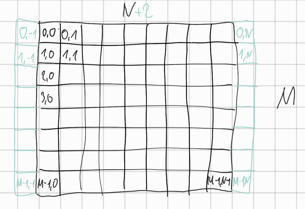
\begin{align} \frac{\partial C }{\partial t} & = \frac{\partial}{\partial x} \left(\alpha \frac{\partial C }{\partial x} \right) \nonumber \\ & = \alpha \frac{\partial^2 C}{\partial x^2} \end{align}

We aim at numerically solving eqn:1 on a spatial grid such as:

/max/tug/src/commit/39ce2a62c3a2aeea0ecf461e6ef702a46a59d361/doc/grid_pqc.pdf

The left boundary is defined on $x=0$ while the center of the first cell - which are the points constituting the finite difference nodes - is in $x=dx/2$, with $dx=L/n$.

The explicit FTCS scheme (as in PHREEQC)

We start by discretizing eqn:1 following an explicit Euler scheme and specifically a Forward Time, Centered Space finite difference.

For each cell index $i \in 1, \dots, n-1$ and assuming constant $\alpha$, we can write:

\begin{equation}\displaystyle \frac{C_i^j+1 -C_i^j}{Δ t} = α\frac{\frac{C^j_i+1-C^j_i}{Δ x}-\frac{C^j_i-C^j_i-1}{Δ x}}{Δ x}

\end{equation}

In practice, we evaluate the first derivatives of $C$ w.r.t. $x$ on the boundaries of each cell (i.e., $(C_{i+1}-C_i)/\Delta x$ on the right boundary of the i-th cell and $(C_{i}-C_{i-1})/\Delta x$ on its left cell boundary) and then repeat the differentiation to get the second derivative of $C$ on the the cell centre $i$.

This discretization works for all internal cells, but not for the domain boundaries ($i=0$ and $i=n$). To properly treat them, we need to account for the discrepancy in the discretization.

For the first (left) cell, whose center is at $x=dx/2$, we can evaluate the left gradient with the left boundary using such distance, calling $l$ the numerical value of a constant boundary condition:

\begin{equation}\displaystyle \frac{C_0^j+1 -C_0^j}{Δ t} = α\frac{\frac{C^j₁-C^j₀}{Δ x}- \frac{C^j₀-l}{\frac{Δ x}{2}}}{Δ x}

\end{equation}

This expression, once developed, yields:

\begin{align}\displaystyle C_0^j+1 & = C_0^j + \frac{α ⋅ Δ t}{Δ x^2} ⋅ ≤ft( C^j₁-C^j₀- 2 C^j₀+2l \right) \nonumber
& = C_0^j + \frac{α ⋅ Δ t}{Δ x^2} ⋅ ≤ft( C^j₁- 3 C^j₀ +2l \right)

\end{align}

In case of constant right boundary, the finite difference of point $C_n$ - calling $r$ the right boundary value - is:

\begin{equation}\displaystyle \frac{C_n^j+1 -C_n^j}{Δ t} = α\frac{\frac{r - C^j_n}{\frac{Δ x}{2}}- \frac{C^j_n-C^j_n-1}{Δ x}}{Δ x}

\end{equation}

Which, developed, gives

\begin{align}\displaystyle C_n^j+1 & = C_n^j + \frac{α ⋅ Δ t}{Δ x^2} ⋅ ≤ft( 2 r - 2 C^j_n -C^j_n + C^j_n-1 \right) \nonumber
& = C_n^j + \frac{α ⋅ Δ t}{Δ x^2} ⋅ ≤ft( 2 r - 3 C^j_n + C^j_n-1 \right)

\end{align}

If on the right boundary we have closed or Neumann condition, the left derivative in eq. eqn:5 becomes zero and we are left with:

\begin{equation}\displaystyle C_n^j+1 = C_n^j + \frac{α ⋅ Δ t}{Δ x^2} ⋅ (C^j_n-1 - C^j_n)

\end{equation}

A similar treatment can be applied to the BTCS implicit scheme.

Implicit BTCS scheme

First, we define the Backward Time difference:

\begin{equation} \frac{\partial C^{j+1} }{\partial t} = \frac{C^{j+1}_i - C^{j}_i}{\Delta t} \end{equation}

Second the spatial derivative approximation, evaluated at time level $j+1$:

\begin{equation} \frac{\partial^2 C^{j+1} }{\partial x^2} = \frac{\frac{C^{j+1}_{i+1}-C^{j+1}_{i}}{\Delta x}-\frac{C^{j+1}_{i}-C^{j+1}_{i-1}}{\Delta x}}{\Delta x} \end{equation}

Taking the 1D diffusion equation from eqn:1 and substituting each term by the equations given above leads to the following equation:

\begin{align}\displaystyle \frac{C_i^j+1 - C_i^j}{Δ t} & = α\frac{\frac{C^j+1_i+1-C^j+1_i}{Δ x}-\frac{C^j+1_i-C^j+1_i-1}{Δ x}}{Δ x} \nonumber
& = α\frac{C^j+1_i-1 - 2C^j+1_i + C^j+1_i+1}{Δ x^2}

\end{align}

This only applies to inlet cells with no ghost node as neighbor. For the left cell with its center at $\frac{dx}{2}$ and the constant concentration on the left ghost node called $l$ the equation goes as followed:

\begin{equation}\displaystyle \frac{C_0^j+1 -C_0^j}{Δ t} = α\frac{\frac{C^j+1₁-C^j+1₀}{Δ x}- \frac{C^j+1₀-l}{\frac{Δ x}{2}}}{Δ x}

\end{equation}

This expression, once developed, yields:

\begin{align}\displaystyle C_0^j+1 & = C_0^j + \frac{α ⋅ Δ t}{Δ x^2} ⋅ ≤ft( C^j+1₁-C^j+1₀- 2 C^j+1₀+2l \right) \nonumber
& = C_0^j + \frac{α ⋅ Δ t}{Δ x^2} ⋅ ≤ft( C^j+1₁- 3 C^j+1₀ +2l \right)

\end{align}

Now we define variable $s_x$ as followed:

\begin{equation} s_x = \frac{\alpha \cdot \Delta t}{\Delta x^2} \end{equation}

Substituting with the new variable $s_x$ and reordering of terms leads to the equation applicable to our model:

\begin{equation}\displaystyle -C^j_0 = (2s_x) ⋅ l + (-1 - 3s_x) ⋅ C^j+1_0 + s_x ⋅ C^j+1_1

\end{equation}

TODO

• Right boundary
• Tridiagonal matrix filling

Old stuff

Input

• c $\rightarrow c$

  • containing current concentrations at each grid cell for species
  • size: $N \times M$
  • row-major

• alpha $\rightarrow \alpha$

  • diffusion coefficient for both directions (x and y)
  • size: $N \times M$
  • row-major

• boundary_condition $\rightarrow bc$

  • Defines closed or constant boundary condition for each grid cell
  • size: $N \times M$
  • row-major

Internals

• A_matrix $\rightarrow A$

  • coefficient matrix for linear equation system implemented as sparse matrix
  • size: $((N+2)\cdot M) \times ((N+2)\cdot M)$ (including ghost zones in x direction)
  • column-major (not relevant)

• b_vector $\rightarrow b$

  • right hand side of the linear equation system
  • size: $(N+2) \cdot M$
  • column-major (not relevant)

• x_vector $\rightarrow x$

  • solutions of the linear equation system
  • size: $(N+2) \cdot M$
  • column-major (not relevant)

Calculation for $\frac{1}{2}$ timestep

Symbolic addressing of grid cells

Filling of matrix $A$

• row-wise iterating with $i$ over c and \alpha matrix respectively
• addressing each element of a row with $j$

• matrix $A$ also containing $+2$ ghost nodes for each row of input matrix $\alpha$

  • $\rightarrow offset = N+2$
  • addressing each object $(i,j)$ in matrix $A$ with $(offset \cdot i + j, offset \cdot i + j)$

Rules

$s_x(i,j) = \frac{\alpha(i,j)*\frac{t}{2}}{\Delta x^2}$ where $x$ defining the domain size in x direction.

For the sake of simplicity we assume that each row of the $A$ matrix is addressed correctly with the given offset.

Ghost nodes

$A(i,-1) = 1$

$A(i,N) = 1$

Inlet

$A(i,j) = \begin{cases} 1 & \text{if } bc(i,j) = \text{constant} \\ -1-2*s_x(i,j) & \text{else} \end{cases}$

$A(i,j\pm 1) = \begin{cases} 0 & \text{if } bc(i,j) = \text{constant} \\ s_x(i,j) & \text{else} \end{cases}$

Filling of vector $b$

• each elements assign a concrete value to the according value of the row of matrix $A$

• Adressing would look like this: $(i,j) = b(i \cdot (N+2) + j)$

  • $\rightarrow$ for simplicity we will write $b(i,j)$

Rules

Ghost nodes

$b(i,-1) = \begin{cases} 0 & \text{if } bc(i,0) = \text{constant} \\ c(i,0) & \text{else} \end{cases}$

$b(i,N) = \begin{cases} 0 & \text{if } bc(i,N-1) = \text{constant} \\ c(i,N-1) & \text{else} \end{cases}$

Inlet

$p(i,j) = \frac{\Delta t}{2}\alpha(i,j)\frac{c(i-1,j) - 2\cdot c(i,j) + c(i+1,j)}{\Delta x^2}$

\noindent $p$ is called t0_c inside code

$b(i,j) = \begin{cases} bc(i,j).\text{value} & \text{if } bc(i,N-1) = \text{constant} \\ -c(i,j)-p(i,j) & \text{else} \end{cases}$