tug/doc/ADI_scheme.org

Adi 2D Scheme

Input

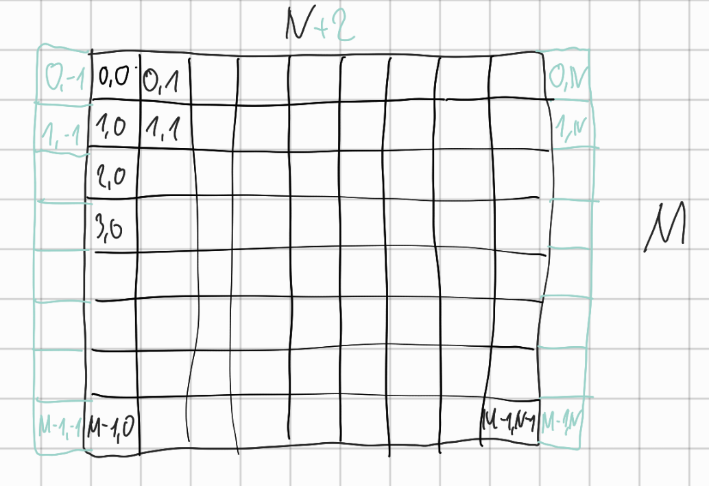
• c $\rightarrow c$

  • containing current concentrations at each grid cell for species
  • size: $N \times M$
  • row-major

• alpha $\rightarrow \alpha$

  • diffusion coefficient for both directions (x and y)
  • size: $N \times M$
  • row-major

• boundary_condition $\rightarrow bc$

  • Defines closed or constant boundary condition for each grid cell
  • size: $N \times M$
  • row-major

Internals

• A_matrix $\rightarrow A$

  • coefficient matrix for linear equation system implemented as sparse matrix
  • size: $((N+2)\cdot M) \times ((N+2)\cdot M)$ (including ghost zones in x direction)
  • column-major (not relevant)

• b_vector $\rightarrow b$

  • right hand side of the linear equation system
  • size: $(N+2) \cdot M$
  • column-major (not relevant)

• x_vector $\rightarrow x$

  • solutions of the linear equation system
  • size: $(N+2) \cdot M$
  • column-major (not relevant)

Calculation for $\frac{1}{2}$ timestep

Symbolic addressing of grid cells

Filling of matrix $A$

• row-wise iterating with $i$ over c and \alpha matrix respectively
• addressing each element of a row with $j$

• matrix $A$ also containing $+2$ ghost nodes for each row of input matrix $\alpha$

  • $\rightarrow offset = N+2$
  • addressing each object $(i,j)$ in matrix $A$ with $(offset \cdot i + j, offset \cdot i + j)$

Rules

$s_x(i,j) = \frac{\alpha(i,j)*\frac{t}{2}}{\Delta x^2}$ where $x$ defining the domain size in x direction.

For the sake of simplicity we assume that each row of the $A$ matrix is addressed correctly with the given offset.

Ghost nodes

$A(i,-1) = 1$

$A(i,N) = 1$

Inlet

$A(i,j) = \begin{cases} 1 & \text{if } bc(i,j) = \text{constant} \\ -1-2*s_x(i,j) & \text{else} \end{cases}$

$A(i,j\pm 1) = \begin{cases} 0 & \text{if } bc(i,j) = \text{constant} \\ s_x(i,j) & \text{else} \end{cases}$

Filling of vector $b$

• each elements assign a concrete value to the according value of the row of matrix $A$

• Adressing would look like this: $(i,j) = b(i \cdot (N+2) + j)$

  • $\rightarrow$ for simplicity we will write $b(i,j)$

Rules

Ghost nodes

$b(i,-1) = \begin{cases} 0 & \text{if } bc(i,0) = \text{constant} \\ c(i,0) & \text{else} \end{cases}$

$b(i,N) = \begin{cases} 0 & \text{if } bc(i,N-1) = \text{constant} \\ c(i,N-1) & \text{else} \end{cases}$

Inlet

$p(i,j) = \frac{\Delta t}{2}\alpha(i,j)\frac{c(i-1,j) - 2\cdot c(i,j) + c(i+1,j)}{\Delta x^2}$¹

$b(i,j) = \begin{cases} bc(i,j).\text{value} & \text{if } bc(i,N-1) = \text{constant} \\ -c(i,j)-p(i,j) & \text{else} \end{cases}$

Finite differences with nodes as cells' centres

The explicit FTCS scheme as in PHREEQC

The 1D diffusion equation is:

\begin{align} \frac{\partial C }{\partial t} & = \frac{\partial}{\partial x} \left(\alpha \frac{\partial C }{\partial x} \right) \nonumber \\ & = \alpha \frac{\partial^2 C}{\partial x^2} \end{align}

We discretize it following a Forward Time, Centered Space finite difference scheme where the nodes correspond to the centers of a grid such as:

/max/tug/src/commit/899e00bec1e5d0ee1139b6d814758efab2d691d0/doc/grid_pqc.pdf

The left boundary is defined on $x=0$ while the center of the first cell is in $x=dx/2$, with $dx=L/n$.

We discretize eqn:1 as following, for each index i in 1, …, n-1 and assuming constant $\alpha$:

\begin{equation}\displaystyle \frac{C_i^j+1 -C_i^j}{Δ t} = α\frac{\frac{C^j+1_i+1-C^j+1_i}{Δ x}-\frac{C^j+1_i-C^j+1_i-1}{Δ x}}{Δ x}

\end{equation}

In practice, we evaluate the first derivatives of $C$ w.r.t. $x$ on the boundaries of each cell (i.e., $(C_{i+1}-C_i)/\Delta x$ on the right boundary of the i-th cell and $(C_{i}-C_{i-1})/\Delta x$ on its left cell boundary) and then repeat the differentiation to get the second derivative of $C$ on the the cell centre $i$.

This discretization works for all internal cells, but not for the boundaries. To properly treat them, we need to account for the discrepancy in the discretization.

For the first (left) cell, whose center is at $x=dx/2$, we can evaluate the left gradient with the left boundary using such distance, calling $l$ the numerical value of a constant boundary condition:

\begin{equation}\displaystyle \frac{C_0^j+1 -C_0^j}{Δ t} = α\frac{\frac{C^j+1₁-C^j+1₀}{Δ x}- \frac{C^j+1₀-l}{\frac{Δ x}{2}}}{Δ x}

\end{equation}

This expression, once developed, yields:

\begin{align}\displaystyle C_0^j+1 & = C_0^j + \frac{α ⋅ Δ t}{Δ x^2} ⋅ ≤ft( C^j+1₁-C^j+1₀- 2 C^j+1₀+2l \right) \nonumber
& = C_0^j + \frac{α ⋅ Δ t}{Δ x^2} ⋅ ≤ft( C^j+1₁- 3 C^j+1₀ +2l \right)

\end{align}

Now we define variable $s_x$ as following:

\begin{equation} s_x = \frac{\alpha \cdot \Delta t}{\Delta x^2} \end{equation}

Substituting with the new variable $s_x$ and reordering of terms leads to the equation applicable to our model:

\begin{equation}\displaystyle -C^j_0} = s_x ⋅ C^j+1_1 + (2s_x) ⋅ l + (-1 - 3s_x) ⋅ C^j+1_0

\end{equation}

In case of constant right boundary, the finite difference of point $C_n$ - calling $r$ the right boundary value - is:

\begin{equation}\displaystyle \frac{C_n^j+1 -C_n^j}{Δ t} = α\frac{\frac{r - C^j_n}{\frac{Δ x}{2}}- \frac{C^j_n-C^j_n-1}{Δ x}}{Δ x}

\end{equation}

Which, developed, gives

\begin{align}\displaystyle C_n^j+1 & = C_n^j + \frac{α ⋅ Δ t}{Δ x^2} ⋅ ≤ft( 2 r - 2 C^j_n -C^j_n + C^j_n-1 \right) \nonumber
& = C_n^j + \frac{α ⋅ Δ t}{Δ x^2} ⋅ ≤ft( 2 r - 3 C^j_n + C^j_n-1 \right)

\end{align}

If on the right boundary we have closed or Neumann condition, the left derivative in eq. eqn:5 becomes zero and we are left with:

\begin{equation}\displaystyle C_n^j+1 = C_n^j + \frac{α ⋅ Δ t}{Δ x^2} ⋅ (C^j_n-1 - C^j_n)

\end{equation}

A similar treatment can be applied to the BTCS implicit scheme.

---

¹

$p$ is called t0_c inside code