tug/doc/ValidationHetDiff.org

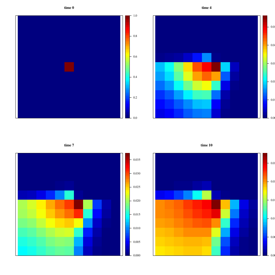
Validation Examples for 2D Heterogeneous Diffusion

Simple setup using deSolve/ReacTran

• Square of side 10
• Discretization: 11 × 11 cells
• All boundaries closed
• Initial state: 0 everywhere, 1 in the center (6,6)
• Time step: 1 s, 10 iterations

The matrix of spatially variable diffusion coefficients α is constant in 4 quadrants:

α_x,y =

0.01	0.01	0.01	0.01	0.01	0.01	0.001	0.001	0.001	0.001	0.001
0.01	0.01	0.01	0.01	0.01	0.01	0.001	0.001	0.001	0.001	0.001
0.01	0.01	0.01	0.01	0.01	0.01	0.001	0.001	0.001	0.001	0.001
0.01	0.01	0.01	0.01	0.01	0.01	0.001	0.001	0.001	0.001	0.001
0.01	0.01	0.01	0.01	0.01	0.01	0.001	0.001	0.001	0.001	0.001
1	1	1	1	1	1	0.1	0.1	0.1	0.1	0.1
1	1	1	1	1	1	0.1	0.1	0.1	0.1	0.1
1	1	1	1	1	1	0.1	0.1	0.1	0.1	0.1
1	1	1	1	1	1	0.1	0.1	0.1	0.1	0.1
1	1	1	1	1	1	0.1	0.1	0.1	0.1	0.1
1	1	1	1	1	1	0.1	0.1	0.1	0.1	0.1

The relevant part of the R script used to produce these results is presented in listing 1; the whole script is at /max/tug/src/commit/8e5c1ad0356fc1cc1dfe3db19b40038f98e5be87/doc/scripts/HetDiff.R. A visualization of the output of the reference simulation is given in figure 1.

Note: all results from this script are stored in the outc matrix by the deSolve function. I stored a different version into /max/tug/src/commit/8e5c1ad0356fc1cc1dfe3db19b40038f98e5be87/scripts/gold/HetDiff1.csv: this file contains 11 columns (one for each time step including initial conditions) and 121 rows, one for each domain element, with no headers.

  library(ReacTran)
  library(deSolve)

  ## harmonic mean
  harm <- function(x,y) {
    if (length(x) != 1 || length(y) != 1)
    stop("x & y have different lengths")
    2/(1/x+1/y)
  }

  N     <- 11          # number of grid cells
  ini   <- 1           # initial value at x=0
  N2    <- ceiling(N/2)
  L     <- 10          # domain side

  ## Define diff.coeff per cell, in  4 quadrants
  alphas <- matrix(0, N, N) 
  alphas[1:N2, 1:N2] <- 1
  alphas[1:N2, seq(N2+1,N)] <- 0.1
  alphas[seq(N2+1,N), 1:N2] <- 0.01
  alphas[seq(N2+1,N), seq(N2+1,N)] <- 0.001

  cmpharm <- function(x) {
    y <- c(0, x, 0)
    ret <- numeric(length(x)+1)
    for (i in seq(2, length(y))) {
      ret[i-1] <- harm(y[i], y[i-1])
    }
    ret
  }

  ## Construction of the 2D grid
  x.grid <- setup.grid.1D(x.up = 0, L = L, N = N)
  y.grid <- setup.grid.1D(x.up = 0, L = L, N = N)
  grid2D <- setup.grid.2D(x.grid, y.grid)
  dx <- dy <- L/N

  D.grid <- list()
  ## Diffusion coefs on x-interfaces
  D.grid$x.int <- apply(alphas, 1, cmpharm)
  ## Diffusion coefs on y-interfaces
  D.grid$y.int <- t(apply(alphas, 2, cmpharm))

  # The model
  Diff2Dc <- function(t, y, parms) {
    CONC  <- matrix(nrow = N, ncol = N, data = y)
    dCONC <- tran.2D(CONC, dx = dx, dy = dy, D.grid = D.grid)$dC
    return(list(dCONC))
  }

  ## initial condition: 0 everywhere, except in central point
  y <- matrix(nrow = N, ncol = N, data = 0)
  y[N2, N2] <- ini  # initial concentration in the central point...

  ## solve for 10 time units
  times <- 0:10
  outc <- ode.2D(y = y, func = Diff2Dc, t = times, parms = NULL,
		 dim = c(N, N), lrw = 1860000)