tug/doc/ADI_scheme.org

Numerical solution of diffusion equation in 2D with ADI Scheme

Finite differences with nodes as cells' centres

The 1D diffusion equation is:

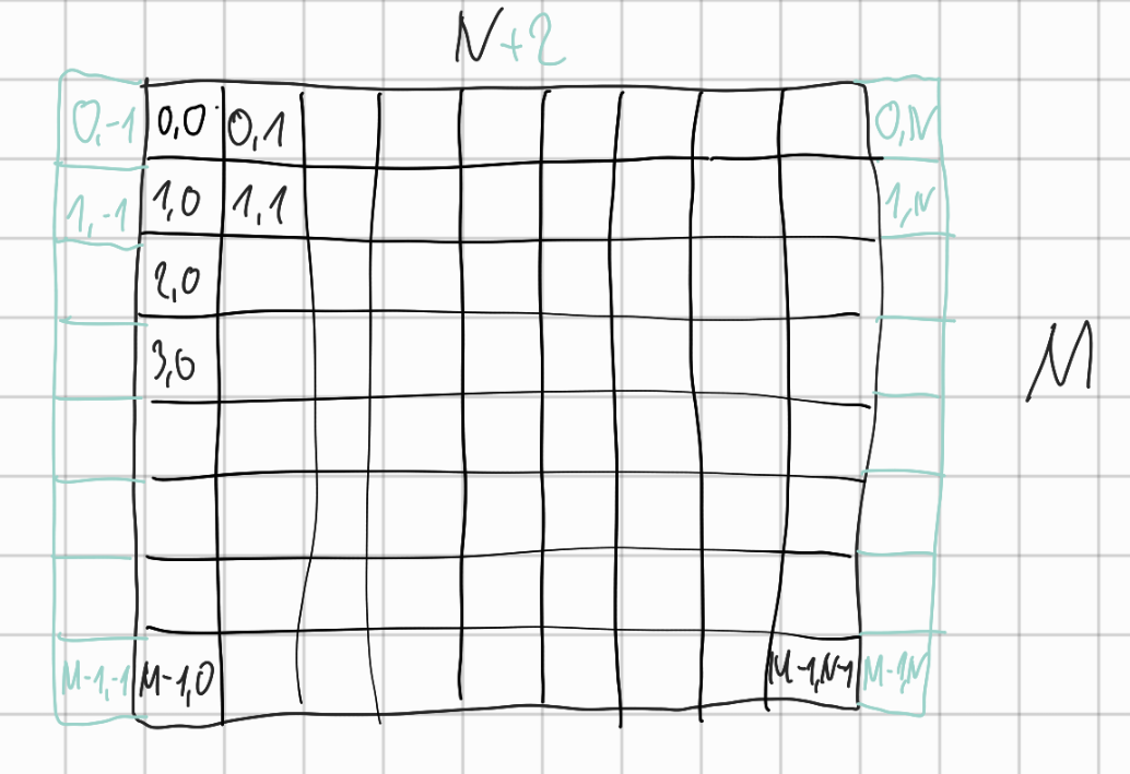
\begin{align} \frac{\partial C }{\partial t} & = \frac{\partial}{\partial x} \left(\alpha \frac{\partial C }{\partial x} \right) \nonumber \\ & = \alpha \frac{\partial^2 C}{\partial x^2} \end{align}

We aim at numerically solving eqn:1 on a spatial grid such as:

/max/tug/src/commit/ffefb6ab50339dde222e27ae4a44b47cbcc9f0e8/doc/grid_pqc.pdf

The left boundary is defined on $x=0$ while the center of the first cell - which are the points constituting the finite difference nodes - is in $x=dx/2$, with $dx=L/n$.

The explicit FTCS scheme (as in PHREEQC)

We start by discretizing eqn:1 following an explicit Euler scheme and specifically a Forward Time, Centered Space finite difference.

For each cell index $i \in 1, \dots, n-1$ and assuming constant $\alpha$, we can write:

\begin{equation}\displaystyle \frac{C_i^j+1 -C_i^j}{Δ t} = α\frac{\frac{C^j_i+1-C^j_i}{Δ x}-\frac{C^j_i-C^j_i-1}{Δ x}}{Δ x}

\end{equation}

In practice, we evaluate the first derivatives of $C$ w.r.t. $x$ on the boundaries of each cell (i.e., $(C_{i+1}-C_i)/\Delta x$ on the right boundary of the i-th cell and $(C_{i}-C_{i-1})/\Delta x$ on its left cell boundary) and then repeat the differentiation to get the second derivative of $C$ on the the cell centre $i$.

This discretization works for all internal cells, but not for the domain boundaries ($i=0$ and $i=n$). To properly treat them, we need to account for the discrepancy in the discretization.

For the first (left) cell, whose center is at $x=dx/2$, we can evaluate the left gradient with the left boundary using such distance, calling $l$ the numerical value of a constant boundary condition:

\begin{equation}\displaystyle \frac{C_0^j+1 -C_0^j}{Δ t} = α\frac{\frac{C^j₁-C^j₀}{Δ x}- \frac{C^j₀-l}{\frac{Δ x}{2}}}{Δ x}

\end{equation}

This expression, once developed, yields:

\begin{align}\displaystyle C_0^j+1 & = C_0^j + \frac{α ⋅ Δ t}{Δ x^2} ⋅ ≤ft( C^j₁-C^j₀- 2 C^j₀+2l \right) \nonumber
& = C_0^j + \frac{α ⋅ Δ t}{Δ x^2} ⋅ ≤ft( C^j₁- 3 C^j₀ +2l \right)

\end{align}

In case of constant right boundary, the finite difference of point $C_n$ - calling $r$ the right boundary value - is:

\begin{equation}\displaystyle \frac{C_n^j+1 -C_n^j}{Δ t} = α\frac{\frac{r - C^j_n}{\frac{Δ x}{2}}- \frac{C^j_n-C^j_n-1}{Δ x}}{Δ x}

\end{equation}

Which, developed, gives

\begin{align}\displaystyle C_n^j+1 & = C_n^j + \frac{α ⋅ Δ t}{Δ x^2} ⋅ ≤ft( 2 r - 2 C^j_n -C^j_n + C^j_n-1 \right) \nonumber
& = C_n^j + \frac{α ⋅ Δ t}{Δ x^2} ⋅ ≤ft( 2 r - 3 C^j_n + C^j_n-1 \right)

\end{align}

If on the right boundary we have closed or Neumann condition, the left derivative in eq. eqn:5 becomes zero and we are left with:

\begin{equation}\displaystyle C_n^j+1 = C_n^j + \frac{α ⋅ Δ t}{Δ x^2} ⋅ (C^j_n-1 - C^j_n)

\end{equation}

A similar treatment can be applied to the BTCS implicit scheme.

Implicit BTCS scheme

First, we define the Backward Time difference:

\begin{equation} \frac{\partial C^{j+1} }{\partial t} = \frac{C^{j+1}_i - C^{j}_i}{\Delta t} \end{equation}

Second the spatial derivative approximation, evaluated at time level $j+1$:

\begin{equation} \frac{\partial^2 C^{j+1} }{\partial x^2} = \frac{\frac{C^{j+1}_{i+1}-C^{j+1}_{i}}{\Delta x}-\frac{C^{j+1}_{i}-C^{j+1}_{i-1}}{\Delta x}}{\Delta x} \end{equation}

Taking the 1D diffusion equation from eqn:1 and substituting each term by the equations given above leads to the following equation:

\begin{align}\displaystyle \frac{C_i^j+1 - C_i^j}{Δ t} & = α\frac{\frac{C^j+1_i+1-C^j+1_i}{Δ x}-\frac{C^j+1_i-C^j+1_i-1}{Δ x}}{Δ x} \nonumber
& = α\frac{C^j+1_i-1 - 2C^j+1_i + C^j+1_i+1}{Δ x^2}

\end{align}

This only applies to inlet cells with no ghost node as neighbor. For the left cell with its center at $\frac{dx}{2}$ and the constant concentration on the left ghost node called $l$ the equation goes as followed:

\begin{equation}\displaystyle \frac{C_0^j+1 -C_0^j}{Δ t} = α\frac{\frac{C^j+1₁-C^j+1₀}{Δ x}- \frac{C^j+1₀-l}{\frac{Δ x}{2}}}{Δ x}

\end{equation}

This expression, once developed, yields:

\begin{align}\displaystyle C_0^j+1 & = C_0^j + \frac{α ⋅ Δ t}{Δ x^2} ⋅ ≤ft( C^j+1₁-C^j+1₀- 2 C^j+1₀+2l \right) \nonumber
& = C_0^j + \frac{α ⋅ Δ t}{Δ x^2} ⋅ ≤ft( C^j+1₁- 3 C^j+1₀ +2l \right)

\end{align}

Now we define variable $s_x$ as followed:

\begin{equation} s_x = \frac{\alpha \cdot \Delta t}{\Delta x^2} \end{equation}

Substituting with the new variable $s_x$ and reordering of terms leads to the equation applicable to our model:

\begin{equation}\displaystyle -C^j_0 = (2s_x) ⋅ l + (-1 - 3s_x) ⋅ C^j+1_0 + s_x ⋅ C^j+1_1

\end{equation}

The right boundary follows the same scheme. We now want to show the equation for the rightmost inlet cell $C_n$ with right boundary value $r$:

\begin{equation}\displaystyle \frac{C_n^j+1 -C_n^j}{Δ t} = α\frac{\frac{r-C^j+1_n}{\frac{Δ x}{2}}- \frac{C^j+1_n-C^j+1_n-1}{Δ x}}{Δ x}

\end{equation}

This expression, once developed, yields:

\begin{align}\displaystyle C_n^j+1 & = C_n^j + \frac{α ⋅ Δ t}{Δ x^2} ⋅ ≤ft( 2r - 2C^j+1_n - C^j+1_n + C^j+1_n-1 \right) \nonumber
& = C_0^j + \frac{α ⋅ Δ t}{Δ x^2} ⋅ ≤ft( 2r - 3C^j+1_n + C^j+1_n-1 \right)

\end{align}

Now rearrange terms and substituting with $s_x$ leads to:

\begin{equation}\displaystyle -C^j_n = s_x ⋅ C^j+1_n-1 + (-1 - 3s_x) ⋅ C^j+1_n + (2s_x) ⋅ r

\end{equation}

TODO

• Tridiagonal matrix filling

2D ADI using BTCS scheme

In the previous sections we described the usage of FTCS and BTCS on 1D grids. To make usage of the BTCS scheme we are following the alternating-direction implicit method. Therefore we make use of second difference operator defined in equation eqn:secondderivative in both $x$ and $y$ direction for half the time step $\Delta t$. We are denoting the numerator of equation eqn:1DBTCS as $\delta^2_x C^n_{ij}$ and $\delta^2_y C^n_{ij}$ respectively with $i$ the position in $x$, $j$ the position in $y$ direction and $n$ as the current time step:

\begin{align}\displaystyle δ^2_x C^n_ij &= Cⁿ_i-1,j - 2Cⁿ_i,j + Cⁿ_i+1,j \nonumber
δ^2_y C^n_ij &= Cⁿ_i,j-1 - 2Cⁿ_i,j + Cⁿ_i,j+1

\end{align}

Assuming a constant $\alpha_x$ and $\alpha_y$ in each direction the equation can be defined:

\begin{align}\displaystyle \frac{C^n+1/2_ij-C^n_ij}{\frac{Δ t}{2}} &= α_x \frac{≤ft( δ^2_x C^n+1/2_ij + δ^2_y Cⁿ_ij\right)}{Δ x^2} \nonumber
\frac{Cⁿ⁺¹_ij-C^n+1/2_ij}{\frac{Δ t}{2}} &= α_y \frac{≤ft( δ^2_x C^n+1/2_ij + δ^2_y Cⁿ⁺¹_ij\right)}{Δ y^2}

\end{align}

Now we will define $s_x$ and $s_y$ respectively as followed:

\begin{align}\displaystyle s_x &= \frac{α_x ⋅ \frac{Δ t}{2}}{Δ x^2} \nonumber
s_y &= \frac{α_y ⋅ \frac{Δ t}{2}}{Δ y^2}

\end{align}

Equation eqn:genADI, once developed in the $x$ direction, yields:

\begin{align}\displaystyle \frac{C^n+1/2_ij-C^n_ij}{\frac{Δ t}{2}} &= α_x \frac{≤ft( δ^2_x C^n+1/2_ij + δ^2_y Cⁿ_ij\right)}{Δ x^2} \nonumber
\frac{C^n+1/2_ij-C^n_ij}{\frac{Δ t}{2}} &= α_x \frac{≤ft( δ^2_x C^n+1/2_ij \right)}{Δ x^2} + α_x \frac{≤ft(δ^2_y Cⁿ_ij\right)}{Δ x^2} \nonumber
C^n+1/2_ij-C^n_ij &= s_x δ^2_x C^n+1/2_ij + s_x δ^2_y Cⁿ_ij \nonumber
-C^n_ij - s_x δ^2_y Cⁿ_ij &= C^n+1/2_ij + s_x δ^2_x C^n+1/2_ij \nonumber
-C^n_ij - s_x ≤ft(C^n_i,j-1-2C^n_i,j+C^n_i,j+1 \right)&= C^n+1/2_ij + s_x ≤ft( C^n+1/2_i-1,j - 2C^n+1/2_i,j + C^n+1/2_i+1,j \right)

\end{align}

All values on the left side of the equation are known and we are solving for $C^{1/2}$. The calculation in $y$ direction for another $\frac{\Delta t}{2}$ is similar and can also be easily derived. Therefore we do not show it here.

TODO:

• ADI at boundaries

Old stuff

Input

• c $\rightarrow c$

  • containing current concentrations at each grid cell for species
  • size: $N \times M$
  • row-major

• alpha $\rightarrow \alpha$

  • diffusion coefficient for both directions (x and y)
  • size: $N \times M$
  • row-major

• boundary_condition $\rightarrow bc$

  • Defines closed or constant boundary condition for each grid cell
  • size: $N \times M$
  • row-major

Internals

• A_matrix $\rightarrow A$

  • coefficient matrix for linear equation system implemented as sparse matrix
  • size: $((N+2)\cdot M) \times ((N+2)\cdot M)$ (including ghost zones in x direction)
  • column-major (not relevant)

• b_vector $\rightarrow b$

  • right hand side of the linear equation system
  • size: $(N+2) \cdot M$
  • column-major (not relevant)

• x_vector $\rightarrow x$

  • solutions of the linear equation system
  • size: $(N+2) \cdot M$
  • column-major (not relevant)

Calculation for $\frac{1}{2}$ timestep

Symbolic addressing of grid cells

Filling of matrix $A$

• row-wise iterating with $i$ over c and \alpha matrix respectively
• addressing each element of a row with $j$

• matrix $A$ also containing $+2$ ghost nodes for each row of input matrix $\alpha$

  • $\rightarrow offset = N+2$
  • addressing each object $(i,j)$ in matrix $A$ with $(offset \cdot i + j, offset \cdot i + j)$

Rules

$s_x(i,j) = \frac{\alpha(i,j)*\frac{t}{2}}{\Delta x^2}$ where $x$ defining the domain size in x direction.

For the sake of simplicity we assume that each row of the $A$ matrix is addressed correctly with the given offset.

Ghost nodes

$A(i,-1) = 1$

$A(i,N) = 1$

Inlet

$A(i,j) = \begin{cases} 1 & \text{if } bc(i,j) = \text{constant} \\ -1-2*s_x(i,j) & \text{else} \end{cases}$

$A(i,j\pm 1) = \begin{cases} 0 & \text{if } bc(i,j) = \text{constant} \\ s_x(i,j) & \text{else} \end{cases}$

Filling of vector $b$

• each elements assign a concrete value to the according value of the row of matrix $A$

• Adressing would look like this: $(i,j) = b(i \cdot (N+2) + j)$

  • $\rightarrow$ for simplicity we will write $b(i,j)$

Rules

Ghost nodes

$b(i,-1) = \begin{cases} 0 & \text{if } bc(i,0) = \text{constant} \\ c(i,0) & \text{else} \end{cases}$

$b(i,N) = \begin{cases} 0 & \text{if } bc(i,N-1) = \text{constant} \\ c(i,N-1) & \text{else} \end{cases}$

Inlet

$p(i,j) = \frac{\Delta t}{2}\alpha(i,j)\frac{c(i-1,j) - 2\cdot c(i,j) + c(i+1,j)}{\Delta x^2}$

\noindent $p$ is called t0_c inside code

$b(i,j) = \begin{cases} bc(i,j).\text{value} & \text{if } bc(i,N-1) = \text{constant} \\ -c(i,j)-p(i,j) & \text{else} \end{cases}$